Wednesday, August 29

Integral properties and definition


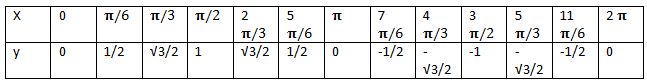
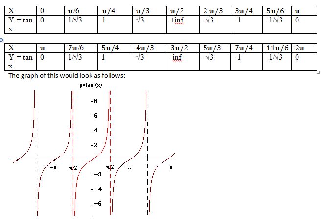
In this article first we define Integration, in mathematics it is an important concept. Its inverse definition is also equally important. Integration is one of the main operations from two basic operations of calculus. In simple form we can define that integration means to calculate area. Now we define mathematically, suppose we have a given function (f) with real variable (x) over an interval [a, b] for a given real line, then we expressed this function as ∫f(x) dx. Integration means calculation of area of the region in XY-plane, which is bounded by the graph of function (x). Area above from the X-axis adds the total value and area below the X-axis subtracts from the total value.

The term integrals also known as antiderivatives. Suppose we have a given function is (F) and derivative of this function is (f). In this case it is known as indefinite integral and can be expressed as ∫f(x) dx. The notion of antiderivative are basic tools of calculus. It has many applications in science and field of engineering. Integral is an infinite sum of rectangles of infinite width. Integral is based on limiting procedure of area. Line integral means function with two or three variables where closed interval are replaced by any curve. Curve may be made in any plane or space. In surface integral in place of plane a short piece of surface is used.

There are various integral properties; integral properties are for the definite notion of antiderivative based on the certain theorems. First theorem is, suppose M(x) and N(x) are two defined functions. They are also continuous function in interval [a, b], then we have linearity property for the notion of antiderivative which can be expressed as
∫ [M(x) +N(x)] dx= ∫M(x) dx + ∫N(x) dx
∫a. M(x) dx= a∫M(x) dx. a is an arbitrary constant and we carry out the constant term from the function.
Second theorem is, suppose function f(x) is defined which is continuous in closed interval [a, b], then we have some special property of integral such as…
∫f(x) dx= 0, when limit are same.
∫f(x) dx= ∫f(x) dx+∫f(x) dx, when limits are divided between interval s like a to c and c to b.
∫f(x) dx= -∫f(x) dx, when upper limit becomes lower limit and lower limit becomes upper limit.

There are many integral types such as definite integral in which function is continuous and define in a closed interval. Other types are indefinite integrals, surface integrals, double integral known as Green’s theorem, triple integrals known as Gauss divergence theorem and line integrals

Monday, August 27

Graphing Trig functions


Sine graph equation:
The general form of a sine function is like this:
Y = sin x.
As we already know, sine is a periodic function. The period of a sine function is 2 pi. That means each value repeats itself after an interval of 2𝛑 on the x axis. The range of the sin function is from -1 to 1. So the value of sin x would not exceed 1 and would not go below -1 at any point. To be able to plot the graph of the function, let us make a table of values of the sine function.

The graph of the above table would look like a wave.

Cosine graph equation:
Just like the sine function, the cosine function is also periodic. The parent cosine function would be like this:
y = cos x
Similar to the sine function, the range of the cosine function is also from -1 to 1. The period of the cosine function is also 2𝛑. That means that the value of the function repeats itself after an interval of 2𝛑. To be able to plot the cosine function now let us make a table of values of cos.

The graph of the function would look like this:

How to graph tangent functions?

The tangent function is also a periodic function. However the period of the tangent function is 𝛑. That means the values repeat itself after an interval of ?? on the x axis. The range of the tangent function is –inf to inf. That means that the tangent function can have any real number value. Just like how we did for the sine and the cosine functions, for plotting the tangent function also we shall make a table of values.


Wednesday, August 22

Properties and derivatives of Logarithm functions


Definition of logarithmic function: For any positive number a is not equal to 1, log base a x = inverse of a^x. The graph of y = log x can be obtained by reflecting the graph of y = a^x across the line y = x. since log x and a^x are inverses of one another, composing them in either order gives the identity function.

We can have some observations about the logarithmic functions. From the graph, we can see that Logarithmic function is defined for positive values only and hence its domain is positive real numbers. The range is set of all real numbers. The graph always passes through (1, 0). The graph is increasing as we move from left to right. In the fourth quadrant, the graph approaches y-axis (but never meets it). It is also clear that the graphs of log base a x and a^x are mirror images of each other if y = x is taken as a mirror line.

Properties of Logarithmic Functions:
For any number x > 0 and y > 0, properties of base a logarithms are:
Product rule: log xy = log x + log y,
Quotient rule: log x / y = log x – log y,
Reciprocal rule: log 1 / y = -log y,
Power rule: log x^y = y log x.

Derivative of Logarithmic Functions: We use the following properties in the differentiation of logarithmic functions.
d/dx(e^x) = e^x
d/dx (log x) = 1/x.

Inverse of logarithmic functions : Since ln x and e^x are inverses of one another, we have  e^ln x = x ( all x > 0 ) ln ( e^x ) = x( all x ).

Logarithmic functions examples: Suppose we have to  Evaluate d/dx log base 10 ( 3x + 1 ).
d/dx log base 10 ( 3x + 1 ) = ( 1 / ln 10 ) .
( 1 / ( 3x + 1 ) ) d / dx ( 3x + 1 ) = 3 / [ ( ln 10 ) ( 3x + 1 ) ].

Evaluate integral log base 2 x /x dx.
Solution: integral log base 2 x / x dx = ( 1 / ln 2 ) integral ln x / x = ( 1 / ln 2 ) integral u du = ( 1 / ln 2 ) ( u^2 / 2 ) + C
= ( 1 / ln 2 ) [ ( ln x )^2 / 2 ] + C = ( ln x )^2 / 2 ln 2 + C.

Monday, August 20

Instantaneous rate of change of a function


Suppose we have a linear function such as y = 2x+3. The graph of this function is as follows:


Assume that to be a graph of the distance traveled by a car from home base, such that at time x = 0, the car is 3 miles from home. Now consider two points on the graph P(1,5) and Q(2,7). If we wish to find the rate of change of distance between these two points, we use the formula:
Rate of change = (y2-y1)/(x2-x1) = (7-5)/(2-1) = 2/1 = 2
That was fairly simple. That is because our graph was a straight line. Now suppose if the graph is not a straight line. And it is a curve instead.


The above graph as we see is not a straight line, but it is a curve. This time the co-ordinates of the points P and Q are (1,7) and (2,13) respectively. The average rate of change from P to Q can be found using the same formula above:
Average rate of change = (13-7)/(2-1) = 6/1 = 6. But we call this average rate of change since, it cannot be exact because the line between P and Q is not a straight line.
With this back ground let us now try to understand what is instantaneous rate of change. Now suppose the point Q moves closer and closer to point P, such that the distance between P and Q is infinitesimally small.

Therefore if co-ordinates of P are (x0, f(x0)) then those of Q would be (x0+h, f(x0+h)). Now, as Q moved closer and closer to P, the value of h goes on decreasing till it finally becomes 0 when Q coincides with P. That does not actually happen, h goes on decreasing to an infinitesimally small value. So we say that h tends to 0. Symbolically, h -> 0. Then the rate of change of the function f would be given as:
Rate of change = lim (h->0) [f(x+h) – f(x)]/[x+h – x] = lim(h->0) [f(x+h) - f(x)]/[h]
Stated above is the instantaneous rate of change equation. The term ‘rate of change’ now becomes ‘instantaneous rate of change’. We call it instantaneous because, at the instant when x = x0, the rate of change of the function is given by the limit:
instantaneous rate of change = lim(h->0) [f(x0+h) – f(x0)]/h

Instantaneous rate of change examples:
Find instantaneous rate of change of f(x) = x^2 at x = 4.
Ir = lim(h->0) [f(4+h) – f(4)]/h = lim(h->0)[16+8h+h^2-16]/h = lim(h->0)[8h+h^2]/h = lim(h->0)[h(8+h)]/h = lim(h->0)[8+h] = 8+0 = 8

Monday, August 13

Difference quotient of a function: Tangent lines and their slopes


This section deal with the problem of finding a straight line L that is tangent to a curve C at a point P. Before we go to learning that, let us make a few assumptions to start with (so as to avoid mathematical errors before we come to the end result). C is the graph of a function y = f(x) and this function is continuous over the interval (a,b). The co-ordinates of the point P are (x0,y0) and the point P lies on the curve C so that f(x0) = y0. Also we assume that P is not the end point of C. That means x0 is not equal to a or b. Therefore C extends to some distance on either sides of P.

A reasonable definition of tangency can be stated in terms of limits. If Q is a point on C different from P, then the line through PQ is called a secant line to the curve. This line rotates around P as Q moves along the curve.  If L is a line through P, whose slope is the limit of the slopes of these secant lines PQ as Q approaches P along C (see picture below), then we say that L is tangent to C at P.

Since C is the graph of the function y = (x), then vertical lines can meet C only once. Since P = (x0,f(x0)), a different point Q on the graph must have a different x-co ordinate, say x0+h, where h ? 0. Thus the co-ordinates of Q would be (x0+h, f(x0+h)) and the slope of the line PQ would be:
= (f(x0+h) – f(x0))/h, based on the formula for slope of line joining two points with co-ordinates (x1,y1) and (x2,y2). Slope = m = (y2-y1)/(x2-x1)

So for our line PQ, that would be:
m = (f(x0+h) – f(x0))/(x+h – x) = (f(x0+h) – f(x0))/h

The above expression is called the difference quotient formula or simply the difference quotient of a function f. Note that h can be positive or negative based on whether Q is to the right or to the left of P.

This method of finding the difference quotient is further applied in finding the derivative of functions in calculus. The basic limit definition of derivatives stems from this difference quotient.

Given the function y = f(x) and a point x = x0, or given a table of values of f(x) for various values of x, to evaluate the difference quotient and subsequently to simplify the difference quotient, is simple.

Wednesday, August 8

Derivative of Cos II


This function is known as differentiation of trigonometric function with use of calculus and various trigonometry rules.

Derivative of Cos Squared X
Derivative of any trigonometric function that is we have to differentiate the function one time. Here we have to find the derivative of Cos squared X. for this first we know the basic rules of differentiation. And also rules of trigonometry.
Derivative of Cos Squared X means first we write the function in (cosX)^2 , now we have to use chain rule . Take external term derivative from the function and then differentiate the internal term we get (2cosxsinx) with negative sign because one time differentiation of cos function is negative sine function.
Now by using trigonometry rule change the result means -2cosxsinx is replaced with -2sin2x. so finally we get derivative of cos squared x is( -2sin2x).

Derivative of Cos -1
Derivative of Cos-1 means we have to differentiate only cos function and cos-1 is a cos function only. So by differentiating that is derivative of cos-1 is sin-1 with negative sign. We have to differentiate only one time.

Derivative of Inverse Cos
For finding the derivative of inverse Cos we use inverse trigonometric rule and calculus rules. Inverse trigonometric function also called sometime as cyclometric function. They are inverse of trigonometric function with proper domains. These are also used as arcos, arcsin and etc.
Inverse laws are very restricted and we can’t go out of the domains. These are proper subsets of domains. Like if function y=square root of x then we write this function as y^2=x also. Similarly function y=arccos then we write this function as cosy=x also. And then differentiate the function.
Derivative of inverse Cos by differentiating we get 1/square root of (1-x^2).
                                              d/dx (arcos) =1/square root of (1-x^2)

Derivative of Cos X Squared
Derivative of Cos X Squared, we write this function also as y=(Cosx)^2, now we differentiate one time this function with respect to x.  Differentiate the external term we get 2 cosx now differentiate the internal term cosx with respect to x then we get sinx with negative sign. Thus total term by differentiating we get 2sinxcosx with negative sign.
We have to write the result in more accurate form. For this we have to use trigonometric rules. By using these rules we get 2sinxcosx in another form is sin2x.so we use this form.
Finally derivative of Cos X Squared we get 2sinxcosx or sin2x with negative sign.
                                     d/dx(cosx)^2=(-sin2x)

Friday, August 3

Intoduction to Partial derivative


Generally we come across with functions of two or more variables. For example, the area of a rectangle, with sides of length x and y is given by A = xy, which obviously depends on the values of x and y, and so it is a function of two variables. Similarly the volume V of a rectangular parallelepiped having sides x, y and z is given by V = xyz and so it is a function of three variables x, y and z. Generally functions of two, three, …, n variables are denoted by f (x, y), f ( x, y, z),…., f(x1, x2,…,xn) respectively. If u = f(x, y) is a function of two variables x and y, then x and y are called independent variables and u is called the dependent variable.

Partial derivatives: Let f(x, y) be a function of two variables x and y. The partial derivatives of f(x, y) with respect to x is defined as Lim h -> 0 f(x + h, y) – f(x, y) / h. Provided that the limit exists and is denoted by del f/del x. Thus, the partial derivative of f(x, y) with respect to x is its ordinary derivative w.r.t. x when y is treated as a constant. Similarly, the partial differentiation of f(x, y) with respect to y is defined as Lim k -> 0  f(x, y + k) – f(x, y) / k .Provided that limit exists and is denoted by del f/del y.

Thus, the partial differentiation of f(x, y) with respect to y is its ordinary derivative w.r.t. y when x is treated as a constant. The process of finding partial differentiation of a function is known as partial differentiation.

Let us see some Partial derivative examples: If f(x, y) = x^3 + y^3 – 3 axy, then Del f/del x = 3 x^2 + 0 – 3 ay = 3 ( x^2 – ay) [because y is treated as a constant].And del f/del y = 0 + 3 y^2 – 3 ax = 3 (y^2 – ax) [because x is treated as a constant].

Partial derivative symbols: Let f(x, y) be a function of two variables such that its partial differentiation (del f/del x) and del f/del y both exists. Then del f/del x and del f/del y are functions of x and y, so we may further differentiate them partial with respect to x or y. The partial differentiation  of del f/del x with respect to x and y are denoted by del^2 f/del x^2 and del^2 f/(del y del x). Similarly, the partial differentiation of del f/del y with respect to x and y are denoted by del^2 f/(del x del y) and del^2 f/del y^2.